
Welcome back to The RAG Learning Log.
In our last two posts, we laid the groundwork with a Basic RAG pipeline and explored how LangChain acts as the glue. But recently, while working on a deeper RAG project, I hit the inevitable glass ceiling. I realized that the "Hello World" approach just wasn't cutting it for real-world complexity—my chunks were breaking context, and my retrievals were often missing the mark. It became obvious that there had to be better techniques and more robust strategies to handle these edge cases. I simply couldn't rely on the "Naïve" approach anymore.
This shift in perspective made me realize that building a RAG pipeline is actually a System Design problem. You aren't just calling APIs; you are architecting a system that needs to balance precision, recall, and latency. Today, we are going to explore that advanced architecture. We’ll look at upgrading our data ingestion with Semantic Chunking, treating user input as a routing challenge with strategies like Decomposition and HyDE, and finally, overhauling our retrieval engine with Hybrid Search and Reranking.
It’s time to stop just finding something and start engineering a system that finds the right thing.
Data Ingestion
Data Chunking Strategies
When I built my first RAG pipeline, I used the industry standard: Recursive Character Text Splitting. It’s the "Ol' Reliable" of LangChain. It tries to be smart by splitting on paragraphs (\n\n) first, then lines (\n), then spaces, aiming to keep structural blocks together.
The Problem: Structure ≠ Meaning.
Concepts don't care about paragraph breaks. I was seeing chunks that cut off right before the "punchline" of a sentence, or separated a pronoun (e.g., "It results in...") from the noun it referred to in the previous chunk.
I needed a strategy that respected the semantics of the text.
The Upgrade: Semantic Chunking
Semantic Chunking doesn't care about characters; it cares about topic shifts. It uses embeddings to measure how "far apart" two sentences are in meaning.
The Mechanics of the "Cosine Check":
Imagine every sentence in your document is a point on a graph.
-
Sentence Embeddings: We pass every sentence through an embedding model (like OpenAI
text-embedding-3-small). This turns the sentence "The sky is blue" into a vector (a list of numbers). -
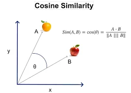
Sequential Comparison: We compare Sentence 1 to Sentence 2, Sentence 2 to Sentence 3, and so on. We calculate the Cosine Similarity between them (a score from 0 to 1, where 1 means identical meaning).
-
The Threshold (The "Break"):
-
If Sentence A and B have a similarity of 0.85, they are talking about the same thing. Keep them together.
-
If Sentence B and C drop to 0.40, the topic has likely shifted (e.g., from "Product Features" to "Legal Disclaimer").
-
This drop is the breakpoint. The splitter cuts the chunk right there.
-
This guarantees that a chunk contains one coherent thought, regardless of whether it is 100 characters or 1000 characters long.
Alternative Strategy: Parent Document Retrieval
Sometimes, Semantic Chunking isn't enough. You face a "Goldilocks" problem:
-
Small chunks are great for retrieval (vector search finds the exact match easily).
-
Large chunks are essential for generation (the LLM needs context to write a good answer).
Parent Document Retrieval (also called Small-to-Big Retrieval) solves this by decoupling what you search from what you send.
How the Architecture Works:
-
The Split: You break your document into massive "Parent" chunks (e.g., 2000 chars).
-
The Sub-Split: You take each Parent chunk and shatter it into tiny "Child" chunks (e.g., 200 chars).
-
The Indexing:
-
You index the Child chunks in the Vector Store (for search).
-
Crucially, you tag each Child with a
parent_idmetadata field. -
You store the full Parent chunks in a separate Doc Store (like Redis or a simple InMemoryStore).
-
-
The Retrieval Time Magic:
-
The user asks a question.
-
Vector search finds the top 5 relevant Child chunks.
-
Instead of returning those fragments, the system looks up their
parent_id, fetches the full Parent chunk from the Doc Store, and feeds that huge context to the LLM.
-
It’s the best of both worlds: the precision of a sniper (finding the exact sentence) with the context of a historian (reading the whole page).
Query Enhancement
Now that our data is beautifully chunked and indexed, we face the next bottleneck: the user.
In a perfect world, users would type keyword-rich, context-heavy queries like "Retrieve the specific safety protocols for the hydraulic press model X-10." In reality, they type: "How do I fix it?"
If you feed that vague, three-word string directly into a vector search, you get garbage results. The "garbage in, garbage out" rule applies to queries just as much as data. I realized that before I could search for the answer, I had to fix the question.
1. Query Transformation & Decomposition
The first line of defense is simply rewriting the user's intent.
-
Transformation (The Rewrite): This is critical for chat applications.
-
The Failure Mode: A user asks "How much does it cost?" The vector store searches for "cost" and returns generic pricing pages for everything you sell.
-
The Fix: We pass the chat history (last 3 turns) and the latest question to an LLM before retrieval. The LLM rewrites the query to: "What is the subscription cost of the Enterprise Plan mentioned in the previous message?" Now, the vector search has a specific target.
-
-
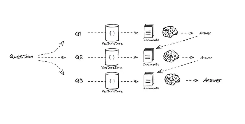
Decomposition (The Break-Down): Vector search struggles with multi-part reasoning.
-
The Failure Mode: If a user asks "Compare the battery life of the iPhone 15 and the Galaxy S24," the embedding for that sentence ends up being a weird mathematical average of "iPhone" and "Samsung." It often retrieves generic documents that mention both brands but lack specific battery details.
-
The Mechanics: We use an LLM (typically a smaller, faster one) to decompose the complex query into sub-queries. The prompt instructs: "Break this down into single-variable questions."
-
Sub-Query A: "What is the battery life of the iPhone 15?" → Executes Search A.
-
Sub-Query B: "What is the battery life of the Galaxy S24?" → Executes Search B.
-
-
The Synthesis: We take the context from Search A and Search B, combine them, and feed them to the LLM to generate the final comparison.
-
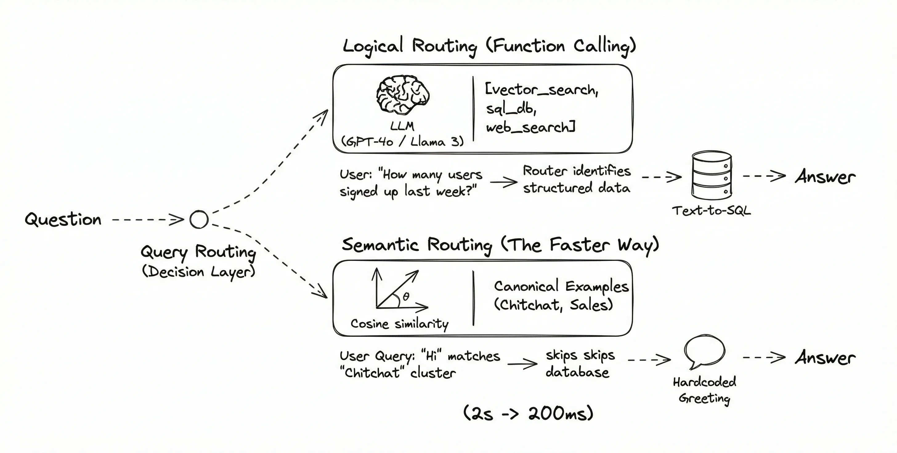
2. Query Routing (The Air Traffic Controller)
Not every question needs to go to the Vector Store. In fact, sending every query there is a waste of money and latency.
Query Routing acts as the decision layer.
-
Logical Routing (Function Calling): We can use an LLM with tool-calling capabilities (like GPT-4o or a fine-tuned Llama 3). We give it a list of tools:
[vector_search, sql_db, web_search].-
User: "How many users signed up last week?"
-
Router: Sees "how many" and "last week," identifies this as a structured data request, and routes to Text-to-SQL.
-
-
Semantic Routing (The Faster Way): Instead of an LLM call (which is slow), we can use embeddings.
-
We create a list of "canonical example queries" for each route (e.g., "Hi", "Hello" for Chitchat; "Price", "Cost" for Sales).
-
When a user query comes in, we check its cosine similarity against these examples. If it matches the "Chitchat" cluster, we skip the database entirely and just reply with a hardcoded greeting. This cuts latency from 2s to 200ms.
-
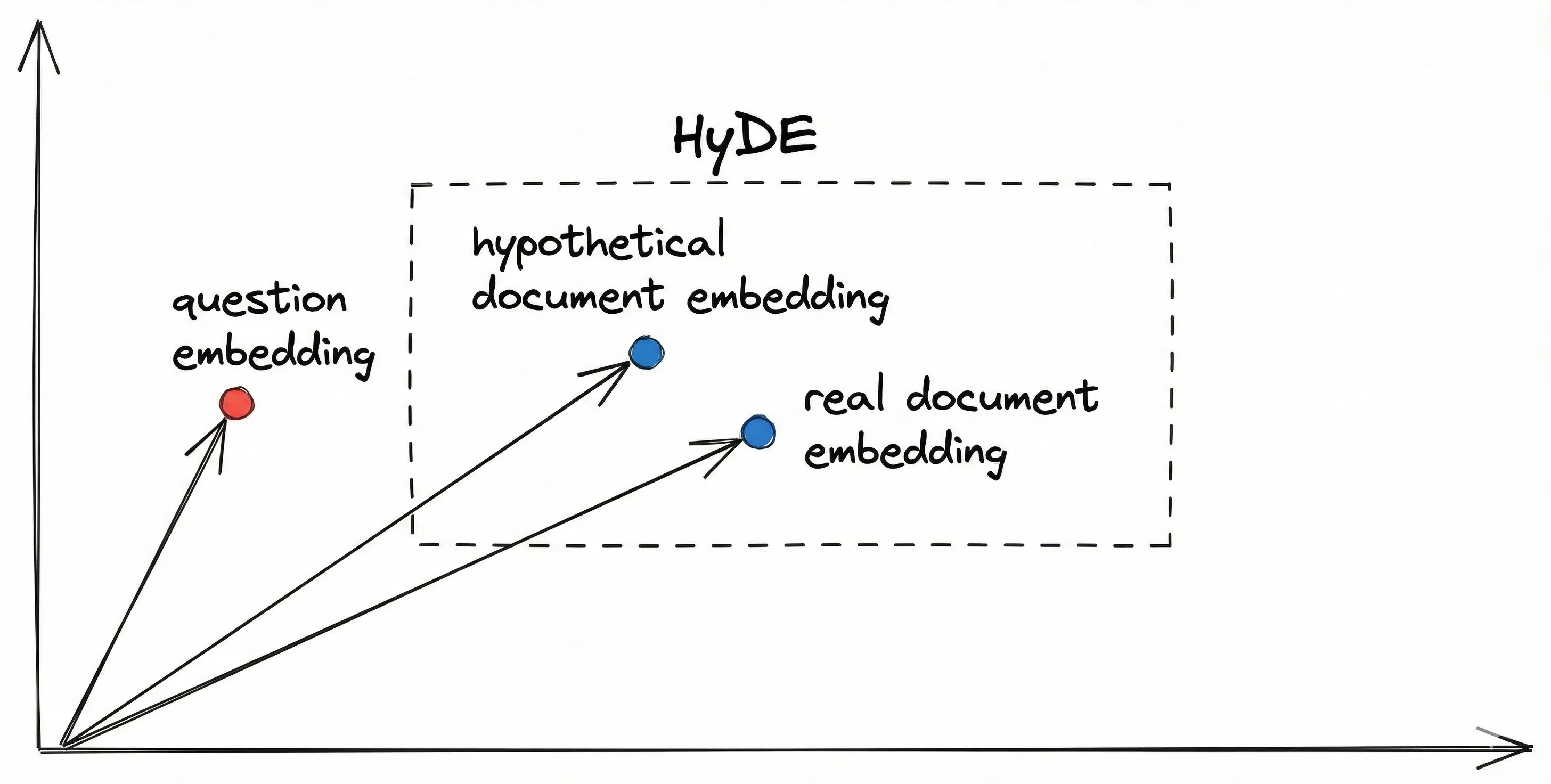
3. HyDE (Hypothetical Document Embeddings)
This is my favorite technique because it feels like "Inception." It solves the vocabulary mismatch problem.
-
The Problem:
-
User Query: "How do I turn on the device?"
-
Actual Document: "To activate the unit, depress the power switch."
-
The Gap: Notice there is zero keyword overlap. "Turn on" vs. "Activate." "Device" vs. "Unit." In vector space, these two sentences might be far apart, meaning your search fails to find the relevant manual.
-
-
The HyDE Solution:
Instead of searching for the question, we search for a theoretical answer.
-
The Hallucination: We ask an LLM: "Write a hypothetical answer to the question: 'How do I turn on the device?'"
-
The Result: The LLM hallucinates: "To turn on the device, you usually press the power button located on the side..." (This might be factually wrong, but that doesn't matter!)
-
The Swap: We embed this hallucinated paragraph.
-
The Search: We use that embedding to search our real database.
-
-
Why it works: The hallucinated answer ("press the power button") shares the same vocabulary and structure as the real document ("depress the power switch"). By searching with an answer to find an answer, we bridge the semantic gap that the raw question couldn't cross.
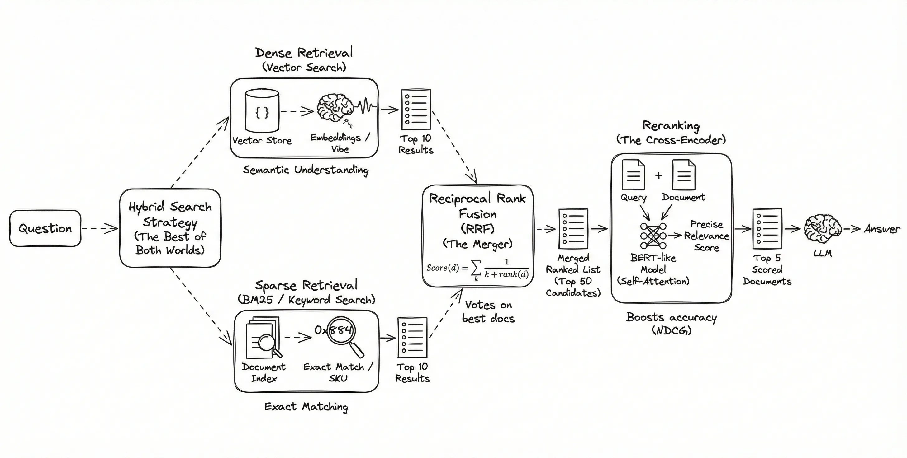
Hybrid Search & Reranking
We have clean chunks (Part 1) and an optimized query (Part 2). Now comes the moment of truth: finding the actual data.
In my early RAG days, I relied 100% on Vector Search (Dense Retrieval). It felt futuristic—you ask a question, and it finds the "vibe" of the answer. But as I moved to production, I ran into the "Specifics Problem."
If a user searched for "Error Code 0x884," the vector search would fail. Why? Because "0x884" doesn't have a semantic meaning in the training data of the embedding model. It’s just a string of characters. The model would return generic error troubleshooting pages, completely missing the specific patch note I needed.
I realized I couldn't abandon the old ways. I needed Hybrid Search.
1. Hybrid Search: The Best of Both Worlds
Hybrid search isn't a single algorithm; it's a strategy of running two distinct search engines in parallel and mathematically merging the results.
-
Dense Retrieval (Vector Search):
-
The Mechanism: Uses embeddings (arrays of floating-point numbers).
-
The Strength: Semantic Understanding. It knows that "canine" is related to "dog" even if the words don't match.
-
The Weakness: It "hallucinates" connections. It might link "Java" (the language) to "Java" (the island) if the context is weak.
-
-
Sparse Retrieval (BM25 / Keyword Search):
-
The Mechanism: This is "Ctrl+F" on steroids. It relies on TF-IDF (Term Frequency-Inverse Document Frequency).
-
The Logic: It rewards documents where your keyword appears frequently (TF), but penalizes words that are common everywhere (like "the" or "and") (IDF).
-
The Strength: Exact Matching. If you search for a unique ID like
SKU-992-X, BM25 will find the exact document containing that string. Vector search often ignores such specific tokens.
-
The Merger: Reciprocal Rank Fusion (RRF)
So, you run both searches. The Vector search gives you its top 10 results. The Keyword search gives you its top 10. How do you combine them into a single, ranked list?
You can't just add the scores because they use different math (Vector is Cosine Similarity 0-1; BM25 is an unbounded score). We use Reciprocal Rank Fusion (RRF).
-
The Philosophy: We don't care about the score; we care about the rank.
-
The Formula: For each document
d, the score is calculated as: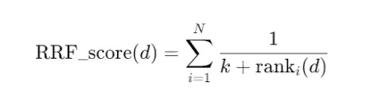
-
Why it works:
-
If Document A is #1 in Keyword search and #1 in Vector search, its score is huge. It bubbles to the top.
-
If Document B is #1 in Keyword but #50 in Vector, it still gets a decent score, respecting the keyword match.
-
It effectively "votes" on the best documents from both perspectives.
-
2. Reranking (The Cross-Encoder)
Even with Hybrid search, we have a bottleneck. Vector stores (like Pinecone or Chroma) rely on Bi-Encoders.
-
The Bi-Encoder Limit: To search fast, the model compresses the document into a vector once (offline) and the query into a vector once (runtime). They never actually "meet" until the comparison. The model misses the subtle interactions between specific words in the query and the document.
-
The Solution: The Cross-Encoder.
A Cross-Encoder doesn't pre-calculate vectors. It takes the Query and the Document as a pair and feeds them into a BERT-like model simultaneously.
-
The Mechanism: It uses a "Self-Attention" mechanism that looks at every word in the query and compares it to every word in the document.
-
The Output: A single score (0 to 1) indicating exactly how relevant that document is to that specific query.
-
The Architecture: Two-Stage Retrieval
We can't use Cross-Encoders for the whole database because they are incredibly slow (100x slower than vector search). So we use a Two-Stage approach:
-
Stage 1 (Retrieval): Use the fast Bi-Encoder (Vector/Hybrid) to retrieve the top 50 candidates. We cast a wide net to ensure we don't miss anything.
-
Stage 2 (Reranking): Pass those 50 candidates through the slow, precise Cross-Encoder.
-
Selection: Take the top 5 scored documents from the Reranker and send only those to the LLM.
Result: This typically boosts accuracy (NDCG scores) by 10-20% because the Reranker filters out the "semantically similar but actually irrelevant" chunks.
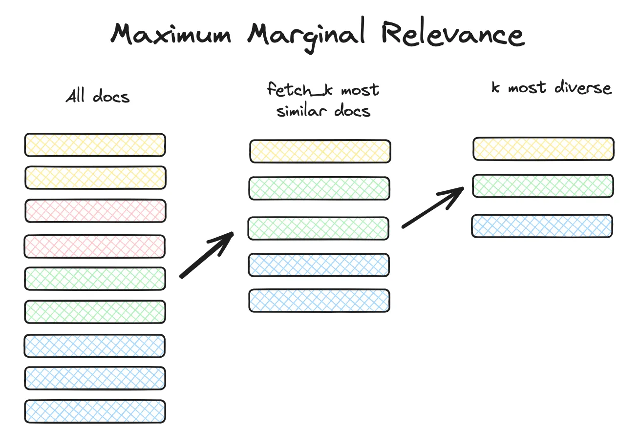
3. Maximal Marginal Relevance (MMR)
Finally, there is the issue of Redundancy.
If I ask "Tell me about the political history of Rome," a standard search might return 5 chunks that are almost identical (e.g., 5 paragraphs from the same textbook chapter). The LLM receives 5 versions of the same fact and misses out on the broader context.
MMR solves this by optimizing for Diversity.
-
The Logic: It selects documents based on a combined score of Relevance (match to query) and Novelty (difference from already selected documents).
-
The "Lambda" ($\lambda$) Knob:
-
If λ = 1 Pure relevance (standard search).
-
If λ = 0: Pure diversity (random distinct topics).
-
The Sweet Spot: We usually set λ = 0.5
-
-
The Algorithm in Action:
-
Pick the single most relevant document (Doc A).
-
For the second slot, look for a document that is relevant to the query MINUS its similarity to Doc A.
-
This ensures the second result covers a new angle of the topic.
-
The Good News: You Don't Have to Build This from Scratch
If reading about Reciprocal Rank Fusion formulas and Cross-Encoder architectures made you sweat, here is the good news: LangChain has already abstracted most of this away.
You don't need to write the math for RRF or manually manage the reranking logic. Almost every technique we discussed maps directly to a pre-built LangChain class.
Here is your "Cheat Sheet" for implementing the Advanced Stack:
1. For Hybrid Search: EnsembleRetriever
Instead of writing complex logic to merge search results, LangChain provides the EnsembleRetriever.
-
How it works: You create a list of retrievers (e.g., your standard
VectorStoreRetrieverand a keyword-basedBM25Retriever). -
The Magic: You pass them into the
EnsembleRetrieveralong with a list ofweights(e.g.,[0.5, 0.5]). When you call.invoke(), it automatically runs all of them, normalizes their scores, and applies the Reciprocal Rank Fusion (RRF) algorithm to give you a single, ranked list.
2. For Reranking: ContextualCompressionRetriever
This name is a mouthful, but it’s the standard wrapper for "Two-Stage Retrieval."
-
The Logic: It takes two arguments:
-
base_retriever: Your initial fast search (the "Stage 1" wide net). -
base_compressor: The model that filters the results.
-
-
The Implementation: You can import
CrossEncoderReranker(backed by Hugging Face models like BGE-Reranker) and pass it as the compressor. LangChain handles the pipeline: it fetches the docs, passes them to the reranker, and returns only the top N results to your chain.
3. For Diversity: .as_retriever(search_type="mmr")
You don't need a special class for Maximal Marginal Relevance. It is built natively into almost every vector store integration (Pinecone, Chroma, FAISS).
-
The Trick: When turning your vector store into a retriever, just swap the search type:
Python
retriever = vectorstore.as_retriever( search_type="mmr", search_kwargs={'k': 5, 'lambda_mult': 0.5} ) -
The Knob: That
lambda_multis your diversity slider. Set it to0.2for wild variety, or0.8for strict relevance.
4. For Semantic Chunking: SemanticChunker
This is available in the langchain_experimental package.
-
How to use: You initialize it with your embedding model (e.g.,
OpenAIEmbeddings()). -
The Flow: You pass your raw text to it just like any other splitter. It internally runs the embeddings, calculates the cosine similarity "breakpoints" we discussed in Part 1, and returns your semantically coherent chunks.
5. For Query Decomposition: MultiQueryRetriever
If you want to break down complex questions, use MultiQueryRetriever.
- What it does: You give it an LLM and your base retriever. Behind the scenes, it prompts the LLM to "generate 3 different versions of this question," retrieves documents for all of them, and dedupes the results (taking the union).
When I started this series, RAG felt like a simple feature: Embed documents → Search → Answer.
But after diving into these advanced techniques, I’ve realized that RAG is not just a feature—it is an architecture. We have effectively moved from a "Hello World" script to a robust Information Retrieval System.
By replacing the naive components with engineered solutions, we have completely transformed the pipeline:
-
Ingestion: We swapped blind text splitting for Semantic Chunking that respects the meaning of the data.
-
Input: We stopped trusting raw user queries and utilized Routing and HyDE to decipher actual intent.
-
Retrieval: We moved beyond simple vector "vibes" to Hybrid Search and Reranking, ensuring we find the exact needle in the haystack.
The result is a system that doesn't just guess—it reasons. It turns a chaotic mess of documents into a precise answer engine. And that is the difference between a cool demo and production-ready software.
Peace out. ✌️